Deriving Great-Circle Distance from Latitude and Longitude

background

Recently, I am working on a hardware device that calculates relative position and distance based on the current GPS coordinates by inputting the longitude and latitude of the target.

When checking related algorithms, I found that most of the derivation processes on the Internet are fragmented or give direct conclusions. In order to thoroughly understand the underlying mathematical logic, I decided to re-derive it from scratch and record it systematically.

This article will completely present this derivation process: starting from the establishment of a three-dimensional space rectangular coordinate system, the vector dot product is used to derive the Law of Spherical Cosines (Law of Cosines). In addition, we will also delve into the physical nature of the “accuracy loss” caused by this formula in short-range scenarios, and how to use the half-angle identity to introduce the Haversine formula to correct the error. Finally, I will share how to reduce the amount of calculations through mathematical simplification and streamlined formulas, thereby achieving higher calculation performance.

Simplified model (flat model)

We learned the Euclidean distance formula in high school mathematics, which is used to calculate the distance between two points on the plane. Similarly, when two points on the earth’s surface are relatively close to each other, we can treat this local area as a plane. In this case, we can directly use the Euclidean distance formula.

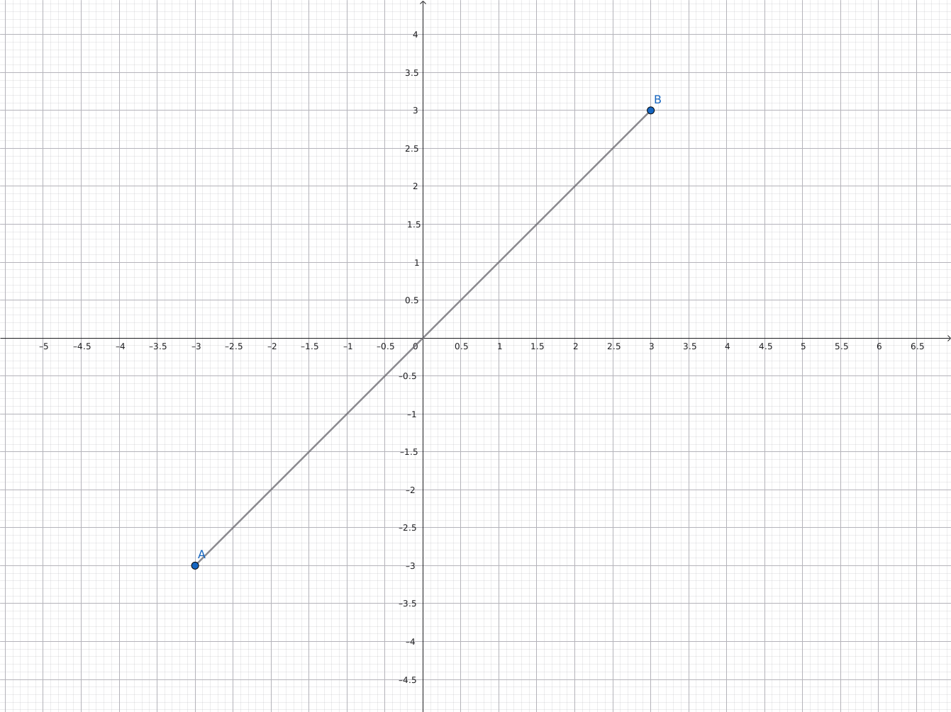
But when two points on the earth’s surface are relatively far apart, we need to consider the curvature of the earth. Below we will introduce how to calculate the distance between two points on the spherical surface.

Spherical model

The real earth is an ellipsoid, and considering the curvature of the earth will increase the complexity of calculations. In most cases, we can simplify the earth into a sphere and obtain a geometric model as shown below.

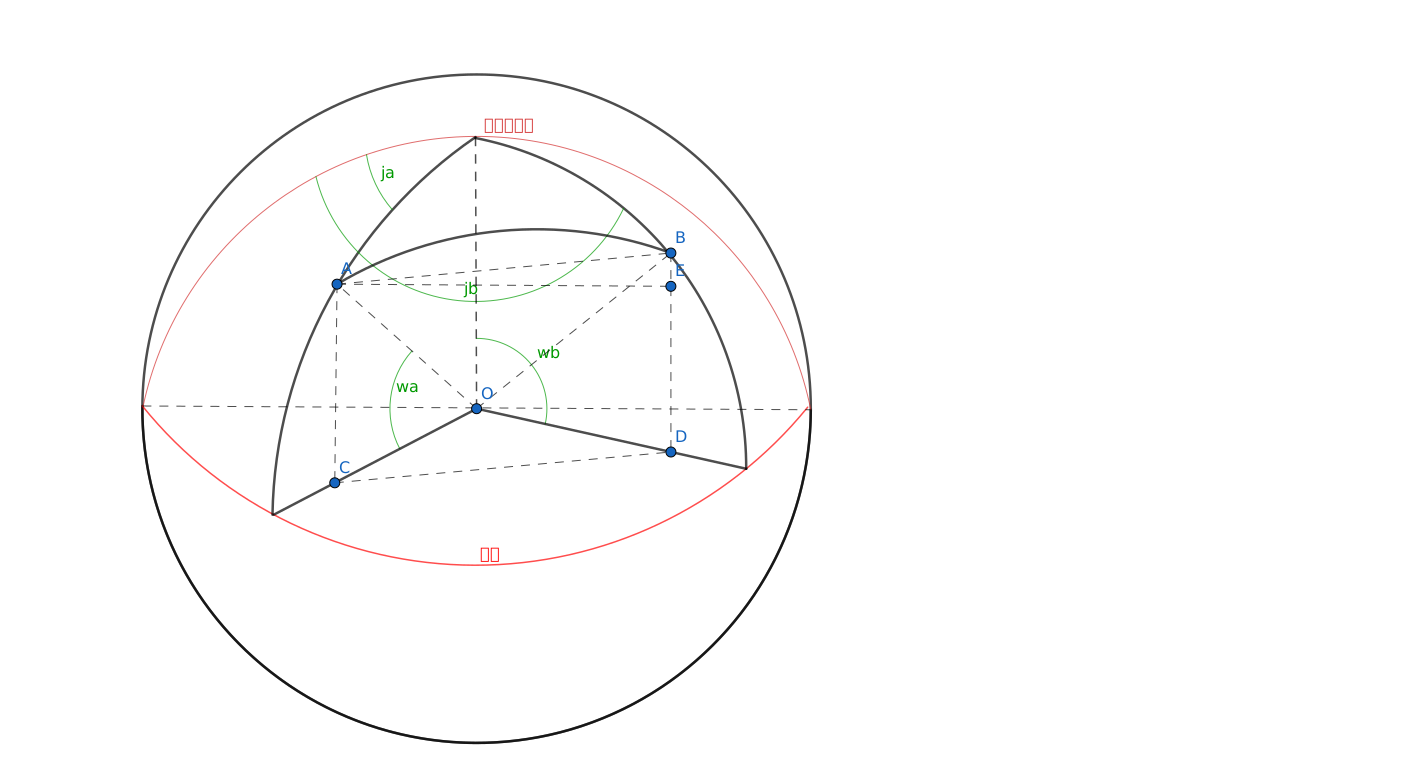
Among them, is the center of the sphere, and are any two points on the sphere, and and are the coordinates of the two points respectively.

Calculate the distance between any two points

To accurately lock the path between the two points and on the sphere, what we are pursuing is the Great Circle Distance, which is the shortest arc length on the sphere.

Geometrically, this distance is the arc length subtended by the central angle : (where is Earth’s radius and is the angle in radians).

The specific solution ideas are as follows:

Three-dimensional coordinate conversion: First convert the two points and to the space rectangular coordinate system through longitude and latitude. Calculate the chord length: Find the length of the straight line segment in three-dimensional space (that is, the base of the triangle ). Reverse the included angle: Use the Law of Cosines to inverse the spherical central angle (hereinafter referred to as ) based on the lengths of the three sides, and then lock the final spherical distance.

The straight-line distance between two points AB can be obtained as Find based on the cosine theorem The form after substituting radius Reverse the formula of According to the arc length formula Substituting gives: Using the formula for derived earlier: Since and , the numerator can be expanded and simplified:

Substitute into the original formula At this point, can be brought into the above parametric equation

After substituting, we get

Extract and get Use formula

The part in brackets can be replaced by the cosine of the longitude difference:

Final formula

This formula is the famous Law of Cosines. The simplified formal logic is clear, and the calculation amount is reduced from 9 trigonometric functions in the derivation process to 6 times, which is very suitable for embedded MCU operation.

Travel notes: The trap of numerical stability (Numerical Stability)

Although this formula is mathematically perfect, in the world of computer floating-point operations, it has a fatal “short board”: When two points are extremely close (such as less than tens of meters), the accuracy will fluctuate violently or even fail completely.

The reason is mainly due to the physical limitations of computers in processing numbers:

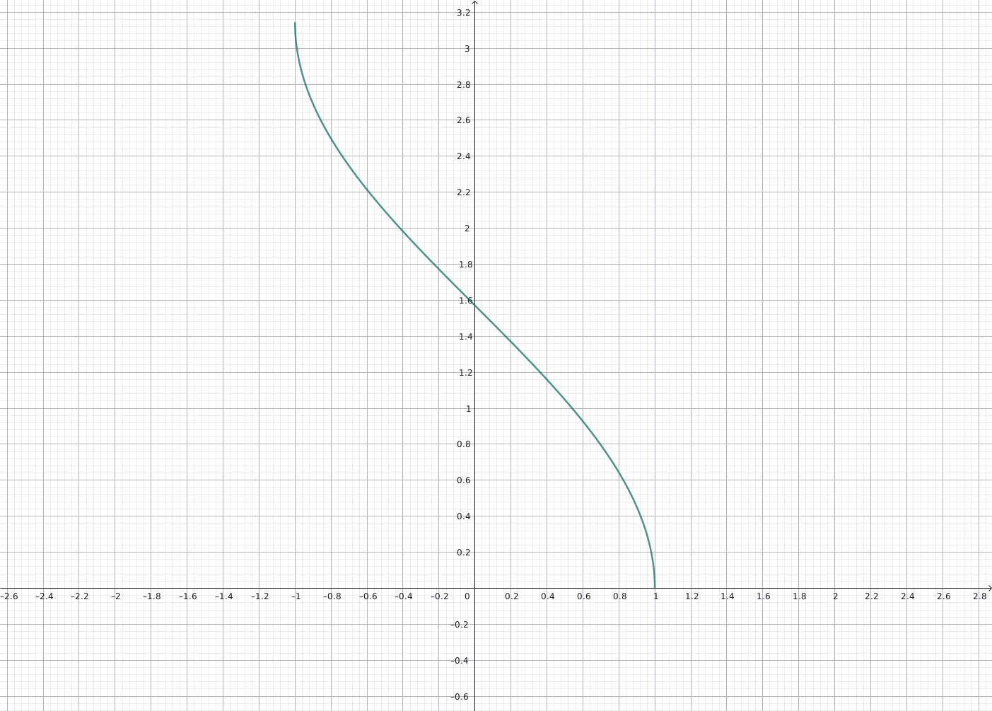
1. The effective accuracy is “squeezed out”: When points A and B are very close, the center angle of the sphere tends to . At this time, the value of will approach infinitely to . Since the upper limit of precision of double-precision floating point numbers (double) is only 15-17 digits, when “1” is used to carry an extremely small offset, the last few significant digits representing the precise offset will be directly truncated.
2. The “death slope” of the arccosine function: Observing the image of we can find (arccos function image) that its derivative near tends to infinity. This means that near , even a very small jitter in the independent variable (such as just the rounding error of the last digit) will be infinitely amplified by the function, causing the calculated distance to “jump repeatedly” between and a huge error value.

In short, for positioning applications that need to deal with short distances (such as a few meters to tens of meters), the law of spherical cosines may directly strike. In order to solve this pitfall, we need to introduce the Haversine formula derived based on the half-angle identity.

Haversine formula

Before introducing the Haversine formula, we first introduce the forward vector function

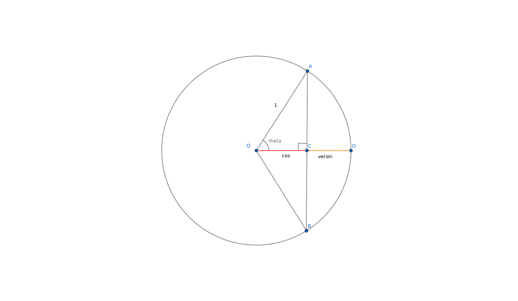
As shown in the figure above, the versine function is called the positive vector function in Chinese and is defined as

The red line segment is , and the orange segment is

Based on the half-angle formula learned in high school

Square both sides to get It is not difficult to find that the right side of the equation is very similar to the definition of the vector function, except that it is divided by 2, so

Based on the transformation of trigonometric identities learned in high school

Through deformation, we can get the form of product and difference:

Now return to the formula of Spherical Cosine Law It is not difficult to find that there is a form of , we can expand it to get Substituting into the formula, we get

Extract the common factor , and get

According to the arc length formula We know that the long string on the right is actually , so

then there is

At this time, both sides are subtracted by 1 at the same time, and we get

A little tidying up

Note that can be rewritten as , then we have Now divide both sides by 2 to get Substitute into the definition of the forward vector function

According to the definition of the semisine function Then the above formula can be written as Taking the square root of both sides gives rule

Substituting the arc length formula again get

After a series of trigonometric function transformations, the final formula is called Haversine formula It solves the problem of numerical stability of spherical cosine law when calculating at close range

In the next article, we will introduce how to calculate the azimuth angle (Bearing) between any two points

References

Using GPS coordinates to calculate distance and azimuth by Johnny Qian

semipositive vector formula